
Economic base analysis divides a region’s activities into basic (export) and nonbasic (local-serving) sectors, then estimates how export-driven jobs support local employment and income. Planners use it to forecast job growth, size infrastructure needs, and justify economic development priorities. The location quotient is the standard tool for the split, but every result needs caveats about productivity, data quality, and time frame before it goes into a report.
TL;DR:
- Location quotients above 4 should be scrutinized carefully to avoid overestimating a sector’s export strength due to productivity differences.
- Using multi-year employment averages and combining multiple methods, such as shift-share and assignment, enhances the reliability of economic base analysis results.
- Data sources like Census CBP, BLS QCEW, and BEA regional accounts are essential for accurate and granular employment analysis at the county or metro level.
- Analysts should validate high-LQ industries locally and consider NAICS aggregation levels at 3- or 4-digit codes to reduce data suppression and compositional bias.
- Results must be presented with clear assumptions, source documentation, and sensitivity tests to ensure transparency and credibility in planning or research contexts.
Table of Contents
- What Is Economic Base Analysis and Why Does It Matter?
- How Do You Calculate a Location Quotient Step by Step?
- What Other Methods Estimate the Economic Base?
- Where Do You Get Reliable Data for a Regional Economic Analysis?
- What Are the Limitations of the Economic Base Model?
- How Do You Build a Reproducible Economic Base Analysis Workflow?
- What Should You Report and What Comes Next?
- Why the Standard Advice on Economic Base Analysis Falls Short
- Sources
What Is Economic Base Analysis and Why Does It Matter?
The theory behind economic base analysis is simple enough to sketch on a napkin: money that comes into a region from outside (exports) circulates locally and pays for goods and services that never leave the area. A factory that ships furniture to another state brings in outside dollars. Those dollars pay wages, and workers spend that money at the local grocery store, the dentist, and the school district. The factory is basic. The grocery store is nonbasic. Grow the basic sector and, in theory, the nonbasic sector follows.
That’s the pitch, and it’s why the method has stuck around in planning offices for decades. It gives you a defensible way to answer questions that show up constantly in local economic development work:
- How many total jobs will a new manufacturing plant support once local spending multiplies through the community?
- Which industries in this county actually export, versus which ones just serve residents who already live here?
- Does this region’s employment mix justify new infrastructure spending, or is growth concentrated in sectors that do not pull outside income?
- How does a proposed real estate development change the local jobs-to-population ratio?
Economic base analysis divides regional activity into basic and nonbasic sectors mainly because sub national trade flows are almost never tracked directly. Nobody publishes county-level export statistics the way the Census Bureau tracks national trade, so analysts infer basic activity from employment patterns instead. Typical basic-to-nonbasic employment ratios run close to 1 to 1, though the ratio swings with region size and economic complexity. Small, single-industry towns skew heavily basic. Large diversified metros trend nonbasic because so much local activity serves the resident population rather than outside buyers.
The method delivers real value when you keep expectations proportional to what employment data can actually show. It’s a screening tool and a conversation starter, not a crystal ball.
How Do You Calculate a Location Quotient Step by Step?
The location quotient formula compares an industry’s share of local employment to that same industry’s share of national employment:
LQ = (local industry employment ÷ total local employment) ÷ (national industry employment ÷ total national employment)
An LQ above 1.0 means the industry employs a larger share of the local workforce than it does nationally, a signal that the industry is likely exporting goods or services beyond the region. The New Mexico State University Extension circular on economic base analysis walks through this exact formula and remains one of the clearest applied references for the calculation.
Here’s the process, start to finish:
- Define your region (county, metro area, or multi-county district) and pick the industry classification level—usually NAICS 3-digit or 4-digit codes—that matches your data’s reliability.
- Pull local employment for the target industry and total local employment across all industries, ideally averaged over two or three years to smooth out seasonal noise.
- Pull national employment for the same industry and the national total, using the same year range and NAICS level.
- Calculate the four ratios and divide the local ratio by the national ratio to get the LQ.
- Flag any industry with LQ > 1.0 as a candidate basic sector, and multiply the “excess” employment (the local jobs beyond what the national ratio would predict) by average wages to estimate export income.
A worked example makes this concrete. Say a county employs 3,000 people in furniture manufacturing out of 60,000 total local jobs. Nationally, furniture manufacturing employs 400,000 people out of 150 million total jobs.
Local ratio: 3,000 ÷ 60,000 = 0.05
National ratio: 400,000 ÷ 150,000,000 = 0.00267
LQ = 0.05 ÷ 0.00267 ≈ 18.7
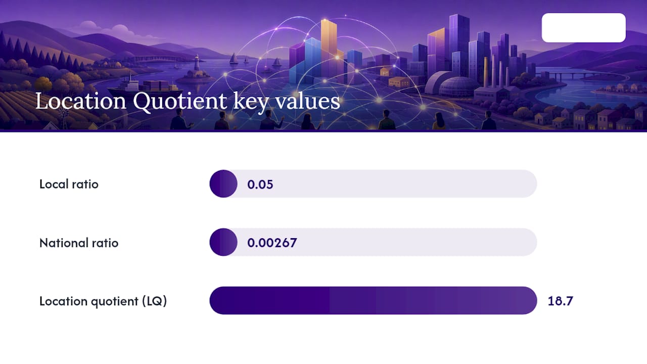
An LQ near 19 signals an extraordinarily concentrated basic industry, the kind you’d expect in a furniture-manufacturing hub. The catch: LQ assumes local and national productivity per worker are identical. If your county’s furniture plants run older equipment and lower output per worker than the national average, you’re overestimating the true export share. Treat any LQ above roughly 3 or 4 with added scrutiny before publishing it as a headline finding.
What Other Methods Estimate the Economic Base?
The location quotient isn’t the only tool, and it isn’t always the right one. Three other approaches show up regularly in applied work, each with a different tradeoff between simplicity and accuracy.
- Assignment method: an analyst manually classifies each industry as basic or nonbasic based on judgment and local knowledge, skipping the math entirely. It’s fast and works when trade data are simply unavailable, but empirical comparisons against regression-based benchmarks show assignment can approximate multipliers reasonably well for many community types while still misjudging the composition of which specific industries are actually export-driven.
- Minimum requirements method: compares your region’s employment share in an industry against the lowest share observed in a set of similar-sized regions, treating anything above that minimum as basic. It avoids the national-average distortion that LQ can introduce, but it depends heavily on picking a sensible comparison set of peer regions.
- Shift-share analysis: decomposes regional job growth into a national growth component, an industry-mix component, and a local competitive component. It doesn’t estimate the base directly, but it tells you whether local growth outpaces what national trends and industry mix alone would predict, useful context alongside an LQ table.
Base multipliers extend all of these methods one step further. A typical multiplier means that each new basic job supports additional nonbasic jobs in the local economy, effectively amplifying the total employment impact, though the exact multiplier varies by region. Multipliers are computed by dividing total employment by basic employment, but treat that number as a snapshot, not a constant. Practitioner research from the Regional Research Institute shows multipliers vary with region type, household income patterns, and local unemployment levels, so a multiplier calculated during a recession can mislead if applied to a recovery-year forecast.
Pick assignment when data are thin and you need a fast qualitative read. Pick LQ when you have reliable employment series and want a repeatable, defensible number. Pick shift-share when the question is about competitiveness rather than the basic/nonbasic split itself.
Where Do You Get Reliable Data for a Regional Economic Analysis?
Every calculation above depends entirely on the quality of the employment data feeding it, and that’s where a lot of student projects and rushed planning reports go wrong.
- County Business Patterns (CBP), published by the Census Bureau, gives establishment counts and employment by NAICS code at the county level, updated annually.
- BLS Quarterly Census of Employment and Wages (QCEW) offers the most granular employment and wage series by industry and county, quarter by quarter.
- BEA regional economic accounts supply income and GDP-by-industry data at the state and metro level, useful for converting employment estimates into dollar terms.
- Census population and commuting products, including American Community Survey commuting flows, help you check whether workers actually live in the region you’re analyzing or commute in from outside it.
NAICS aggregation level matters more than most students expect. A 6-digit NAICS code gives sharp industry detail but suffers from small-sample suppression in rural counties. A 3-digit code avoids suppression but blends dissimilar sub-industries together, sometimes hiding the exact export activity you’re trying to isolate. Extension guidance from New Mexico State University recommends starting at 3-digit or 4-digit NAICS for most county-level work and drilling down only where the data support it.
Two practical fixes solve most data headaches. First, average employment across two or three years rather than relying on a single snapshot, which smooths out one-off layoffs or plant openings. Second, when a cell is suppressed for confidentiality, estimate it using payroll or establishment-count ranges rather than dropping the industry from the analysis entirely.
What Are the Limitations of the Economic Base Model?
No method built on employment counts alone can fully capture a regional economy, and economic base analysis carries specific blind spots worth naming before you present results to a planning commission.
- Static multiplier assumption: the model assumes the basic-to-nonbasic ratio holds steady over the forecast period, when in practice multipliers shift with unemployment, wage levels, and household spending patterns.
- Identical productivity assumption: LQ calculations assume local workers in an industry produce at the same rate as the national average, which frequently isn’t true across regions with different capital investment or labor market age.
- Omitted variables: the model as commonly applied leaves out interregional capital flows, labor migration, and shifts in production technology, all of which can drive local economic change independent of the export base.
- Aggregation bias: choosing too coarse a NAICS level can mask a genuinely export-driven sub-industry inside a larger, mostly local-serving category.
- Commuting and seasonality distortion: a county with heavy in-commuting or a strongly seasonal industry (tourism, agriculture) can show misleading LQ swings depending on which quarter or month the employment data reflect.
Three mitigations handle most of this. Run a sensitivity analysis by recalculating LQs and multipliers under a couple of different NAICS aggregation levels to see how much your conclusions shift. Validate ambiguous industries locally. Construction and specialized business services, in particular, often get misclassified by LQ alone and benefit from a quick local survey or interview to confirm export orientation. And combine methods rather than leaning on LQ in isolation. Pairing an LQ table with a shift-share breakdown gives a planning commission two independent lines of evidence instead of one number that looks more precise than it is.
Pro Tip: Run your LQ calculation twice, once at 3-digit NAICS and once at 4-digit, before you finalize a report. If the “basic” industry list changes significantly between the two, that instability itself is worth reporting to whoever is relying on your numbers.
How Do You Build a Reproducible Economic Base Analysis Workflow?
A defensible economic base analysis isn’t one calculation, it’s a short sequence of decisions that need to be documented well enough that someone else could reproduce your results. Here’s a workflow that holds up under scrutiny from a planning board or a thesis committee alike:
- Define the region precisely, county, metro statistical area, or a custom multi-county district, and state why that boundary makes sense for the question at hand.
- Select the NAICS level for your industry breakdown, and note the tradeoff between detail and suppressed-cell risk explicitly in your methodology section.
- Gather multi-year employment data from CBP, QCEW, and BEA regional accounts, averaging at least two years to reduce single-year noise.
- Compute LQs for every industry in your dataset, not just the ones you expect to be basic, since surprises happen in sectors you weren’t watching.
- Validate locally by checking high-LQ industries against known local business activity, interviews, or trade association data where available.
- Run multiplier scenarios under at least two assumptions (a conservative and an optimistic productivity adjustment) rather than presenting a single point estimate as fact.
Granular, defensible comparators make every step of that workflow stronger, particularly step 5. When Bizminer supplies custom NAICS benchmarks across thousands of markets, you’re checking your LQ-derived basic sector list against real financial and employment patterns for that specific industry code rather than a generic national average. That kind of comparator matters most in step 3 and 5, where an analyst without access to granular NAICS-level benchmarking data has to guess at whether a local anomaly is real or a data artifact.
The deliverable that comes out the other end should include three pieces: a results table showing LQs and multiplier estimates by industry, a written assumptions appendix (NAICS level, years averaged, productivity adjustment used), and a short decision brief translating the numbers into what they mean for the planning question at hand.
What Should You Report and What Comes Next?
Economic base analysis earns its keep when the question is straightforward: which industries bring outside money into this region, and how much local employment does that support? It works less well as a long-range predictive tool, since it ignores capital flows, migration, and shifting production technology over time. Treat every result as a well-documented estimate, not a forecast carved in stone.
Before publishing or presenting results, confirm you’ve covered the basics:
- Named your data sources (CBP, QCEW, BEA) and the years used
- Stated your NAICS aggregation level and why you chose it
- Reported multi-year averages rather than single-year snapshots
- Listed your model’s core assumptions, especially the identical-productivity assumption
- Run at least one sensitivity test on your NAICS level or multiplier assumption
From there, next steps depend on who you are. Students should pair the quantitative LQ work with a short local validation interview or two. Planners should run scenario variants before committing multiplier estimates to a budget document, and consider a follow-up cluster analysis for any industry showing an unusually high LQ, since concentrated industries often cluster with suppliers and specialized labor pools worth tracking separately.
Why the Standard Advice on Economic Base Analysis Falls Short
Most guides treat the location quotient like a finished answer instead of what it actually is: a screening filter. The research backs a narrower claim than most classroom treatments suggest. Isserman’s guidance frames base analysis as a transparent forecasting dialogue with stakeholders, not a standalone predictive model, and that framing gets lost the moment someone drops an LQ table into a report without the assumptions attached.
The bigger blind spot is the export-only mindset. Recent work on regional growth theory makes clear that local clustering and import substitution generate real growth too, independent of exports. A region can grow by getting better at serving itself, not just by selling more outside its borders. Most base analysis writeups never mention that possibility.
If you take one thing from this piece, take this: run the LQ, but spend at least as much effort validating it locally and testing your NAICS aggregation choice as you spent calculating it in the first place. The number is only as good as the decisions behind it.
— Danny
Sources
- Economic base analysis — Wikipedia
- Tools for understanding economic change in communities: Economic base analysis and shift-share analysis — New Mexico State University (CR643)
- Critical assessment of economic base model limitations — University of Chicago repository
- Isserman — guidance on using economic base analysis as a practical planning tool