Retail market analysis is the systematic process of measuring demand, supply, and competitive dynamics within a defined trade area to identify where revenue opportunities exist and where they don’t. The single most valuable action you can take right now: run a trade-area leakage scan using NAICS-level demand estimates against actual retail supply, and you’ll know within an hour whether a market is undersupplied, saturated, or hiding a gap worth pursuing.
What a solid retail market analysis delivers:
- A quantified demand estimate by retail category, tied to real population and income data
- A supply inventory that maps existing competitors by NAICS code and estimated sales volume
- A surplus/leakage calculation that converts the gap into a projected revenue opportunity
- A prioritized hypothesis, ranked by capture-rate potential, that drives the next investment decision
Three steps to start in the next 90 minutes:
- Data check: Pull the latest U.S. Census Bureau American Community Survey data for your target trade area (county or zip code). Confirm population, median household income, and retail expenditure per capita.
- Trade-area leakage scan: Compare estimated retail demand (population × per-capita category spend) against supply (Data Axle or Economic Census sales estimates). Calculate leakage percentage by NAICS category.
- Prioritized hypothesis: Flag the top two or three categories where leakage exceeds 20% and demand is large enough to support a viable store, then frame a testable expansion or recruitment recommendation.
U.S. retail sales remain a multi-trillion-dollar market, and the 2026 outlook continues to reward analysts who can separate genuine demand gaps from noise in the data.
Key Takeaways
A trade-area leakage scan paired with NAICS-level financial benchmarks is the fastest path from raw retail market data to a defensible investment recommendation.
| Point | Details |
|---|---|
| Start with leakage, not headlines | Calculate potential vs. actual sales by six-digit NAICS before drawing any strategic conclusion from national growth figures. |
| Layer your data stack | Combine Census/BLS public data with Data Axle supply inventories and ESRI trade-area mapping before adding financial benchmarks. |
| Run three scenarios | Model conservative, base, and upside capture rates for every white-space opportunity; document all assumptions with data vintage. |
| Operationalize, don’t one-off | Refresh foot-traffic data monthly, supply inventory quarterly, and the full demand model annually to keep analysis current. |
| Bizminer for benchmark depth | Use Bizminer’s granular NAICS benchmarks to validate demand estimates and set format-level performance targets across 9,000+ markets. |
Table of Contents
- What does the U.S. retail market look like heading into 2026?
- What are the core components of retail market analysis?
- How do you run a retail market analysis from start to finish?
- Which data sources and tools should analysts use?
- How should you approach retail forecasting and scenario planning?
- What do retail market analysis deliverables look like?
- How long does a retail market analysis take, and what does it cost?
- How do you govern and operationalize retail market analysis?
- Top actions to take first
- What the data-first approach actually demands
- Bizminer gives analysts the benchmarks that public data can’t
- Sources
What does the U.S. retail market look like heading into 2026?
The U.S. retail sector is one of the largest and most closely tracked markets in the world. Total retail and food service sales have grown steadily through the post-pandemic period, with e-commerce consistently capturing a larger share of total spend each year. The Bureau of Labor Statistics tracks consumer expenditure patterns that feed directly into retail demand models, while the U.S. Census Bureau’s Monthly Retail Trade Survey provides the most current revenue benchmarks by category.
E-commerce now accounts for a meaningful and growing slice of total retail, shifting where demand is captured rather than eliminating it. Brick-and-mortar formats that have survived and grown tend to serve missions e-commerce can’t replicate well: immediate need, tactile experience, and community anchor functions. That distinction matters for any trade-area model because online leakage is real leakage, and ignoring it inflates your demand estimates.
Key metrics to anchor your market snapshot:
- Total U.S. retail revenue: tracked monthly by the Census Bureau’s Monthly Retail Trade Survey, segmented by NAICS category
- Year-on-year growth rate: compare the trailing 12 months against the prior period, adjusted for inflation using BLS CPI data
- E-commerce share: Census Bureau’s Quarterly E-Commerce Report provides the most reliable figure, updated quarterly
- Consumer confidence and credit conditions: Federal Reserve consumer credit data and the Conference Board’s Consumer Confidence Index are leading indicators for discretionary retail
For 2026, the primary demand drivers are real wage growth (which has outpaced inflation in several recent quarters), moderating interest rates, and continued population migration toward Sun Belt metros. Analysts using Deloitte’s annual retail industry outlook and IBISWorld’s sector reports as secondary benchmarks will find consistent signals around grocery, home improvement, and health/personal care as the most resilient categories. Statista aggregates many of these figures into accessible dashboards for quick cross-referencing.
The geographic granularity of your snapshot matters as much as the headline number. Always ground your market snapshot at the trade-area level before drawing any strategic conclusions.
What are the core components of retail market analysis?
Every credible retail market analysis rests on six components. Miss one and your gap calculation will be wrong in a way that’s hard to catch until someone challenges your numbers in a client meeting.
The six core components:
- Trade-area definition: the geographic boundary within which you expect to capture the majority of customer demand. Defined by drive time, distance rings, or natural barriers (highways, rivers, competing anchors).
- Demand estimation: population × per-capita category expenditure, sourced from Census ACS data and consumer expenditure surveys. This is your potential sales figure.
- Supply inventory: a point-level count of existing retailers by NAICS code, with estimated annual sales from Data Axle or the Economic Census. This is your actual sales figure.
- Surplus/leakage analysis: the difference between potential and actual sales. Leakage means residents are spending outside the trade area; surplus means the area draws shoppers from outside. Both have strategic implications.
- Competitive mapping: spatial distribution of competitors, their estimated market share, and any planned openings or closures that would shift supply.
- Consumer behavior signals: shopping frequency, channel preference, demographic composition, and psychographic demand signals that explain why leakage exists, not just that it does.
Key KPIs to collect for every analysis:
- Sales per square foot: total annual sales ÷ gross leasable area (GLA). Industry benchmarks vary sharply by format; Bizminer’s retail trade benchmarks provide NAICS-level comparisons.
- Market penetration rate: your subject store’s sales ÷ total trade-area demand for that category
- Average transaction value (ATV): total revenue ÷ number of transactions; critical for capture-rate modeling
- Footfall proxies: mobile device visit data (from foot-traffic providers) or parking counts as a proxy for store traffic
- Revenue per customer: annual sales ÷ unique customer count; useful for loyalty and frequency analysis
- Pull factor: actual sales ÷ expected sales (based on population share). A pull factor above 1.0 means the area draws outside shoppers; below 1.0 signals leakage.
Example formulae:
Potential sales (demand): Population × Per-capita category expenditure = Potential Sales ($)
Leakage %: (Potential Sales − Actual Sales) ÷ Potential Sales × 100
Pull factor: (Local Sales ÷ State Sales) ÷ (Local Population ÷ State Population)
Trade-area gap analysis, pull-factor calculations, and GIS mapping are the standard methods for identifying surplus and leakage across multiple NAICS levels, and they hold up whether you’re analyzing a rural county or a dense urban corridor.
Pro Tip: Use six-digit NAICS codes whenever your data source supports it. Three-digit codes (e.g., NAICS 445: Food and Beverage Stores) are useful for high-level scans, but six-digit codes (e.g., NAICS 445110: Supermarkets and Other Grocery Stores) reveal the specific category gaps that actually drive site decisions. Mixing levels in the same analysis is one of the most common errors analysts make.
How do you run a retail market analysis from start to finish?
A repeatable workflow keeps your analysis auditable and your team aligned. Here’s the end-to-end sequence, with the data fields and formats you need at each step.

1. Project scoping
Define the business question precisely: site selection, market entry, competitive response, or economic development recruitment. The question determines your trade-area size, NAICS depth, and the level of primary research needed.
2. Trade-area mapping
Draw your trade area using drive-time polygons (5, 10, 20 minutes) or distance rings, depending on the retail category. Grocery draws from a tight 3-mile radius; home improvement pulls from 15+ miles. Use ESRI’s ArcGIS or a comparable GIS platform to generate the polygon and extract the population and demographic data within it.
3. Data collection
Gather the following in parallel:
- Census ACS 5-year estimates (population, income, household size) — available as CSV or API
- Consumer Expenditure Survey (BLS) for per-capita category spend by income band
- Data Axle business list for the trade area (point-level retailers, estimated sales, square footage) — delivered as CSV or shapefile
- Economic Census data for sales benchmarks at the county level (quinquennial, so check vintage)
4. Supply inventory
Map every existing retailer in the trade area by six-digit NAICS code. Record name, address, estimated annual sales, and square footage. Flag any planned openings or closures from local permit data or commercial real estate sources.
5. Demand modeling
Calculate potential sales for each NAICS category: multiply trade-area population by the BLS per-capita expenditure for that category. Adjust for income distribution if your trade area skews significantly above or below the national median.
6. Gap analysis
Subtract actual sales (from your supply inventory) from potential sales. Calculate leakage percentage and pull factor for each category. A market opportunity analysis quantifies unmet demand using addressable population, category spend, and competitor coverage, then converts that unmet demand into revenue via capture-rate assumptions.
Apply the PassBy framework here: Unmet demand × Expected capture rate × ATV = Projected revenue. Run three capture-rate scenarios with conservative, base, and optimistic assumptions to bracket the opportunity.
7. Validation
Cross-check your demand estimates against at least one secondary source (Bizminer benchmarks, IBISWorld, or Statista). Run intercept surveys or shop-along research to validate why leakage is occurring. Primary research methods like intercept surveys, shop-alongs, and NPS tracking complement secondary data when profiling customer segments and refining capture-rate inputs.
8. Recommendations
Translate gap analysis into one of three actions:
- Expansion: leakage >25%, demand large enough to support a viable store, no dominant competitor within the trade area. Recommend site acquisition or lease.
- Recruitment: leakage >20%, but the gap is best filled by attracting an existing regional or national chain rather than a new entrant. Prepare a recruitment package with the leakage data.
- Pilot: leakage is moderate (10–20%), competitive dynamics are uncertain, or the category is shifting online. Recommend a pop-up, kiosk, or limited-format test before full commitment.
Visual outputs to build:
- Trade-area heatmap showing demand density by block group
- Supply-density map with competitor locations and estimated sales radius
- Surplus/leakage table by NAICS category (six-digit, sortable by leakage %)
- KPI dashboard: pull factor, penetration rate, ATV, and sales-per-sq-ft by trade area
Which data sources and tools should analysts use?
The right data stack depends on your budget, geography, and the NAICS depth you need. Here’s how the major sources break down, and where each fits in a practical workflow.
Public data sources
U.S. Census Bureau is the foundation of any demand model. The American Community Survey (ACS) provides annual population, income, and household estimates down to the census tract and block group. The Economic Census (conducted every five years, most recently for 2022) gives sales and establishment counts by NAICS code at the county level. Both are free and available via API or bulk download.
Bureau of Labor Statistics (BLS) supplies the Consumer Expenditure Survey, which is the standard source for per-capita retail spending by category and income band. Updated annually, it’s the numerator in most demand calculations.
Census Bureau’s County Business Patterns (CBP) fills the gap between Economic Census years with annual establishment and payroll data by NAICS, useful for tracking supply-side changes year over year.
Commercial data sources
ESRI (ArcGIS) is the dominant GIS platform for trade-area mapping. It geocodes addresses, generates drive-time polygons, and integrates demographic data directly into the mapping environment. ESRI also sells its own consumer spending estimates (Tapestry segmentation), which some analysts use as an alternative to raw BLS data.
Data Axle provides point-level business lists with estimated annual sales, employee counts, and square footage for individual retail locations. It’s the most practical source for building a supply inventory at the store level, and it’s the source OSU Extension’s retail analysis toolbox specifically recommends for local retail spending estimates and business lists.
Foot-traffic data providers (such as mobile location analytics platforms) give visit counts, dwell time, and cross-shopping patterns at the store level. These are particularly useful for validating footfall proxies and understanding competitive draw.
Where Bizminer fits
Public data gives you the raw inputs. Commercial GIS and business-list providers give you the geographic and supply-side layer. What most analysts are missing is the financial benchmarking layer: how does a specific retail category perform financially at a given revenue scale and geography?
Bizminer’s granular industry financial and market benchmarks cover more than 9,000 markets segmented by NAICS code, geography, and company size. For a retail market analysis, that means you can pull sales-per-sq-ft benchmarks, gross margin ratios, and operating cost structures for the exact retail subcategory you’re analyzing, at the county or metro level. Bizminer data is accepted in U.S. Tax Court and used by government agencies, which matters when your analysis needs to hold up to scrutiny. The platform also offers customizable report templates and API access, so benchmarks can feed directly into your analyst dashboard rather than sitting in a static PDF.
The recommended data stack, in sequence:
- Raw public data: Census ACS + BLS CES + CBP (demand inputs and supply benchmarks)
- Commercial enrichment: Data Axle (store-level supply inventory) + ESRI ArcGIS (trade-area mapping and geocoding)
- Financial benchmarking: Bizminer benchmarks by NAICS and geography (validate demand estimates, set performance targets)
- Analyst dashboard: your BI platform (Tableau, Power BI, or similar) pulling from all three layers
For advanced analytics applications, including machine learning-based segmentation and demand forecasting, AI tools are increasingly integrated into retail analytics workflows to automate pattern detection across large datasets.
Pro Tip: When combining Census and Data Axle figures, always note the vintage of each source in your methodology appendix. The Economic Census is five years old by the time you use it; Data Axle is updated more frequently but uses estimation models for sales figures. Flagging this distinction protects your analysis from the most common credibility challenge.
How should you approach retail forecasting and scenario planning?
Forecasting is where retail market analysis shifts from describing what is to projecting what could be. The method you choose should match the decision being made.
Four forecasting approaches:
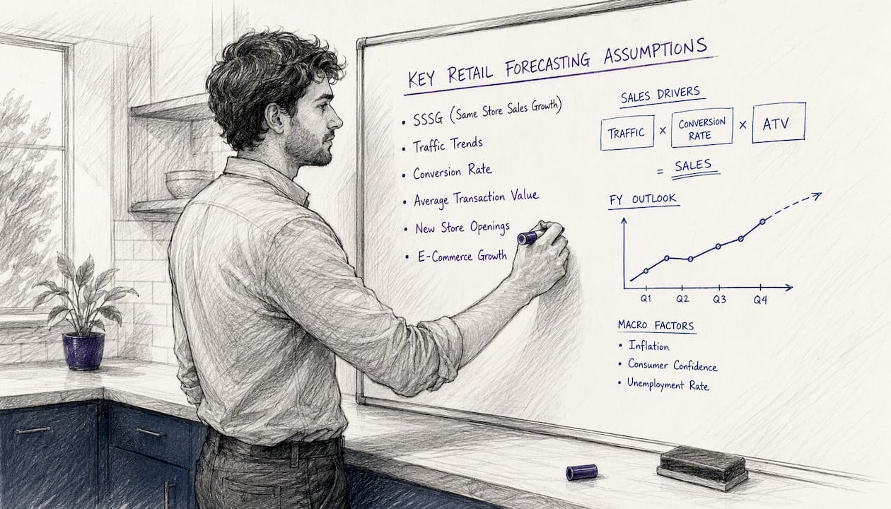
- Baseline trend projection: extend historical sales growth using a compound annual growth rate (CAGR), adjusted for known macro factors (inflation, population change, e-commerce penetration). Best for stable categories with long data histories.
- Top-down TAM→SAM→SOM: start with total addressable market, narrow to serviceable addressable market by geography and format, then estimate share of market. Useful for investor presentations and high-level market entry decisions.
- Bottom-up unit economics: build from store-level assumptions (sq. ft. × sales per sq. ft. × occupancy rate). Bottom-up unit economics are the preferred approach for store-level decisions, while top-down TAM→SAM→SOM works better for high-level sizing and investor pitches.
- Hybrid approach: layer format-level revenue-per-sq-ft benchmarks onto demand-side logic. A hybrid sizing approach, combining demand-side logic with format-level revenue-per-square-foot benchmarks, produces the most actionable estimates for retail expansion decisions.
Scenario planning: base, downside, upside
| Scenario | Key Assumptions | Revenue Impact |
|---|---|---|
| Base | Real wage growth holds, e-commerce share stable, capture rate 15% | Projected revenue at midpoint of demand gap |
| Downside | Consumer credit tightens, unemployment rises 1–2 pts, capture rate 8% | Revenue — below base case |
| Upside | Population inflow accelerates, anchor tenant opens nearby, capture rate 25% | Revenue 30% above base case |
Document every assumption with its data source and vintage. If you’re using BLS CES data from 2024 and ESRI demographic projections for 2026, say so explicitly. Assumptions that aren’t documented become liabilities when the forecast is revisited six months later.
Macro factors to incorporate:
Inflation erodes real consumer spending even when nominal sales grow. Unemployment shifts discretionary spend before it shows up in retail sales data. Consumer credit availability (tracked by the Federal Reserve’s G.19 release) is a leading indicator for big-ticket categories like furniture and electronics. Build these as sensitivity inputs, not fixed assumptions, so stakeholders can see how the forecast moves when conditions change.
Pro Tip: Version your scenario models with a date stamp and the data vintage used. When you update the model in six months, you’ll want to know exactly what changed and why the forecast shifted, rather than reconstructing assumptions from memory.
What do retail market analysis deliverables look like?
A retail market analysis is only as useful as its presentation. Stakeholders who can’t read the output won’t act on it.
Standard deliverable checklist:
- Executive summary (2 pages max): headline findings, top three recommendations, and the leakage/surplus table for the highest-priority categories
- Trade-area maps: demand heatmap, supply-density map with competitor locations, and a combined gap map showing where demand exceeds supply
- Surplus/leakage table: six-digit NAICS categories sorted by leakage percentage, with potential sales, actual sales, and gap in dollars
- KPI dashboard: pull factor, penetration rate, ATV, and sales-per-sq-ft benchmarks versus industry norms, updated to the most recent data vintage
- Scenario table: base/downside/upside projections with assumptions documented
- Appendix: raw data sources, NAICS mapping decisions, formulas used, data vintage for each source, and any primary research instruments
Visual design principles for executive consumption:
Maps should use a single, consistent color scale (darker = higher demand or higher leakage) with a clear legend and scale bar. Avoid layering more than three data variables on a single map. Tables should be sorted by the metric that drives the decision (leakage %, not alphabetically by category). KPI dashboards work best when they show current value, benchmark comparison, and trend direction in a single row per metric.
Business intelligence dashboards transform retail decisions when they’re built around the specific question being answered, not around every metric the data can produce. Resist the temptation to include every KPI you calculated. A dashboard with 30 metrics is a data dump; one with 8 focused metrics is a decision tool.
Sample report outline:
Section 1: Executive Summary. Two pages. Headline market size, top leakage categories, and prioritized recommendations with projected revenue impact.
Section 2: Trade-Area Profile. Demographics, income distribution, population trends, and comparison to state and national benchmarks.
Section 3: Demand Analysis. Potential sales by NAICS category, data sources, and methodology.
Section 4: Supply Inventory. Competitor list, estimated sales, square footage, and market share by category.
Section 5: Gap Analysis. Surplus/leakage table, pull factors, and white-space map.
Section 6: Recommendations. Expansion, recruitment, or pilot recommendation per category, with capture-rate scenarios.
Appendix. Data sources, vintages, NAICS mapping, formulas, and primary research instruments.
How long does a retail market analysis take, and what does it cost?
Project scope drives both timeline and cost more than any other factor. Here’s a realistic breakdown across three common project types.
| Project Type | Timeline | Typical Scope |
|---|---|---|
| Quick scan | 1–2 weeks | Single trade area, 3–5 NAICS categories, public data only |
| Standard analysis | 4–8 weeks | 2–5 trade areas, full NAICS depth, commercial data + GIS |
| In-depth program | 3–6 months | Multi-market, primary research, scenario modeling, ongoing monitoring |
Role responsibilities:
- Data engineer: pulls and cleans Census, BLS, and commercial data; builds the demand model in a reproducible format (Python, R, or SQL)
- GIS analyst: creates trade-area polygons, geocodes supply inventory, and produces all map outputs
- Market analyst: runs the gap analysis, builds scenarios, and writes the narrative
- Stakeholder lead: defines the business question, reviews outputs, and translates recommendations into decisions
Key cost drivers:
- Data licensing (Data Axle business lists, ESRI ArcGIS subscriptions, foot-traffic data)
- GIS platform costs (ESRI licensing scales with user count and data volume)
- Staff time (the largest cost in most projects; GIS and modeling work is time-intensive)
- Custom modeling (machine learning demand forecasting or custom segmentation adds significant time)
- Travel and fieldwork for primary research (intercept surveys, shop-alongs)
Ways to reduce cost without sacrificing quality:
Use public data for the initial scan before committing to commercial data purchases. Run online surveys instead of in-person intercepts for consumer behavior validation. Phase the reporting: deliver a quick-scan leakage table first, then expand to full analysis only for the categories that show genuine opportunity. Sampling a subset of trade areas and extrapolating to similar markets can cut GIS and data costs significantly on multi-market programs.
How do you govern and operationalize retail market analysis?
A one-off analysis is a snapshot. An operationalized program is a competitive advantage. The difference is governance.
Governance checklist:
- Assign a named owner for trade-area definitions. When boundaries change (a new highway opens, a competitor anchor closes), someone needs to be accountable for updating them.
- Establish a benchmark update schedule tied to data vintage. Bizminer benchmarks and Census ACS data have different release cadences; your model should reflect the most current vintage of each.
- Set approval gates for major assumption changes (e.g., adjusting capture-rate inputs requires sign-off from the strategy lead).
- Document every NAICS mapping decision. If you’re using NAICS 445110 for one market and 445 for another, that inconsistency will corrupt any cross-market comparison.
Recommended refresh cadence:
- Monthly: foot-traffic data, consumer confidence indicators, and any real-time sales data available
- Quarterly: competitive supply inventory (new openings, closures, remodels), e-commerce share estimates
- Annually: full demand model refresh using updated ACS and BLS CES data; benchmark recalibration using updated Bizminer or IBISWorld figures
Red flags that signal a compromised analysis:
- Using Economic Census data more than five years old without flagging the vintage
- Mixing three-digit and six-digit NAICS codes in the same leakage table
- Ignoring online channel leakage (treating e-commerce spend as “lost” rather than modeling it as a separate supply category)
- Applying national capture-rate assumptions to a trade area with unusual demographics or competitive dynamics
Market analysis is most effective when embedded as a continuous, cross-departmental function; integrating financial benchmarks into recurring cycles improves both actionability and organizational alignment. That means sharing the leakage table with the real estate team, the benchmark dashboard with the finance team, and the scenario model with the strategy team, rather than keeping the analysis siloed in a single analyst’s folder.
Cross-functional integration also means using financial benchmarking as a shared reference point across planning cycles. When sales, product, and strategy teams are all working from the same NAICS-level benchmarks, the conversation shifts from “what do we think the market can support?” to “here’s what the data says, and here’s where we diverge from it.”
Top actions to take first
Immediate (this week):
- Pull Census ACS data for your target trade area and calculate potential sales for your top three NAICS categories using BLS per-capita expenditure figures.
- Request a Data Axle business list for the same trade area and build your supply inventory.
Near-term (next 30 days):
- Run the full surplus/leakage calculation and pull-factor analysis across all relevant NAICS categories.
- Map the results in ESRI ArcGIS or a comparable GIS tool and identify the top two or three white-space opportunities.
- Validate demand assumptions with at least one round of primary research (intercept surveys or shop-alongs).
Strategic (next quarter):
- Build a scenario model with base/downside/upside projections for each priority category, incorporating macro inputs (inflation, unemployment, consumer credit).
- Establish a governance cadence: monthly foot-traffic refresh, quarterly supply inventory update, annual full model rebuild.
- Integrate Bizminer benchmarks into your reporting template so every analysis includes a NAICS-level financial comparison, not just a demand/supply gap.
The core principle: a trade-area leakage scan paired with Bizminer’s granular benchmarks gives you both the gap and the performance context to make a defensible recommendation, not just a directional one.
What the data-first approach actually demands
Most retail market analyses fail not because the analyst lacked data, but because the analysis was built around a conclusion someone already wanted to reach. The data-first approach means running the leakage calculation before you know which categories will show a gap, and being willing to report that a market is saturated when the numbers say so, even when the client came in expecting an expansion recommendation.
The NAICS granularity question is where this discipline shows up most clearly. Analysts who work at the three-digit level often find apparent gaps that disappear entirely at the six-digit level, because the broad category is undersupplied but the specific format the client operates is already well-covered. Running the analysis at six-digit NAICS from the start, using Bizminer’s customizable benchmark reports to set format-level performance expectations, is what separates an analysis that holds up in a board presentation from one that gets picked apart in the first question.
The other discipline that separates strong analyses from weak ones is transparent assumption documentation. Every capture-rate input, every data vintage, every NAICS mapping decision should be visible in the appendix. When the forecast is revisited in 12 months, the team should be able to reconstruct exactly what was assumed and why the projection moved. That auditability is also what makes Bizminer’s data particularly useful in high-stakes contexts: the platform’s benchmarks are accepted in U.S. Tax Court, which means they carry the kind of documented methodology that survives scrutiny.
Bizminer gives analysts the benchmarks that public data can’t
Running a retail market analysis with public data alone leaves a critical gap: you can calculate the demand/supply difference, but you can’t tell whether the financial performance of existing retailers in that category is strong, weak, or at the margin. That’s the layer Bizminer adds.
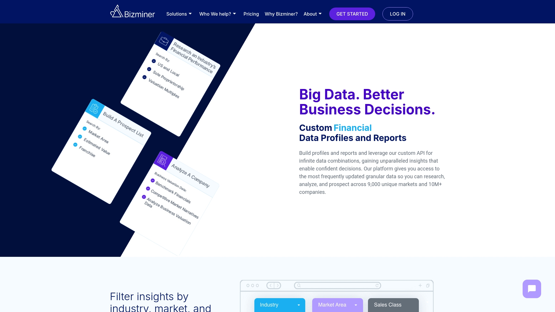
Bizminer covers more than 9,000 markets with granular NAICS-level financial benchmarks, including sales per square foot, gross margin, and operating cost ratios segmented by geography and company size. For an analyst running a leakage analysis, that means you can pair your gap calculation with a benchmark showing what a viable store in that category actually needs to generate to be profitable, not just whether a gap exists. For an advisor producing a custom market report for a client, Bizminer’s customizable report templates and API access mean the deliverable is audit-ready and reproducible, not a one-off spreadsheet that can’t be updated when the data changes.
The platform is used by accounting professionals, business advisors, financial institutions, and government agencies, and its data is accepted in U.S. Tax Court. Start with Bizminer’s market and industry research platform to pull benchmarks for your target NAICS category and geography, and see how your demand estimates compare to what the market is actually producing.
Sources
Public datasets:
- How to Conduct a Market Analysis: A Step-by-Step Guide for Businesses — AMA
- OSU-Extension-Retail-Market-Analysis-to-Wisconsin.pdf
- Market Opportunity Analysis for Retail: How to Size and Prioritize New Markets – PassBy
Commercial and analytical resources: